


Test setup and explanation measurements
Contents


Measuring cables is not easy. That may seem like a crazy statement. Surely it’s super easy to send a “sweep” from 20 Hz to 20 KHz through a cable and see what the deviation is? That is indeed simple. The simplest measuring equipment can do it. However, that doesn’t say anything. And for several reasons.
First of all, all interlinks measure perfectly straight from 20 Hz to 20 KHz. Even up to 100 kHz, the bulk is just straight within less than 0.1 dB. In short: no need to look there. And for those who now say: there you go!…. There is no difference! Take three cables and go listen carefully: there is an audible difference. However, it is not in the frequency response.
Moreover, a sweep is not a simulation of reality: music is many times more complex. There are large and very small dynamics differences and rapid transients. That is a completely different load on a cable than a test tone or sweep.
The question, of course, is: how do you simulate a dynamic piece of music? Honestly: we haven’t been able to do that yet, but we have gained a better understanding of how a cable responds to an extremely fast pulse (we use a pulse with a width of 2ns in our tests). This in a sense simulates the fast transients in music, although the bandwidth required for such a pulse is rather extreme (500 MHz). At least: if you want to reproduce it perfectly. However, that was not the task in this test.
Also, it is crucial that the impedances are correct. For example: the output impedance of a preamplifier is low (say 50 or 100 Ohm … ideally well below 1000 Ohm) and the input impedance of a power amplifier is high (say 10 KOHm or higher). A measuring device usually does not simulate this well, but it is crucial to simulate this situation, otherwise the cable will show a very different behavior.
And as reported, timing behavior in cables is something that few people look at. We tried to give some insight into that by shooting fast pulses through the cable and looking at what the delays are and what the spectrum looks like (resonances, reflections and dampening). This test shows big differences between cables. And we also see a relationship there with sound. Just like in the response measurements up to 10 MHz, by the way. More about that later.
The black box
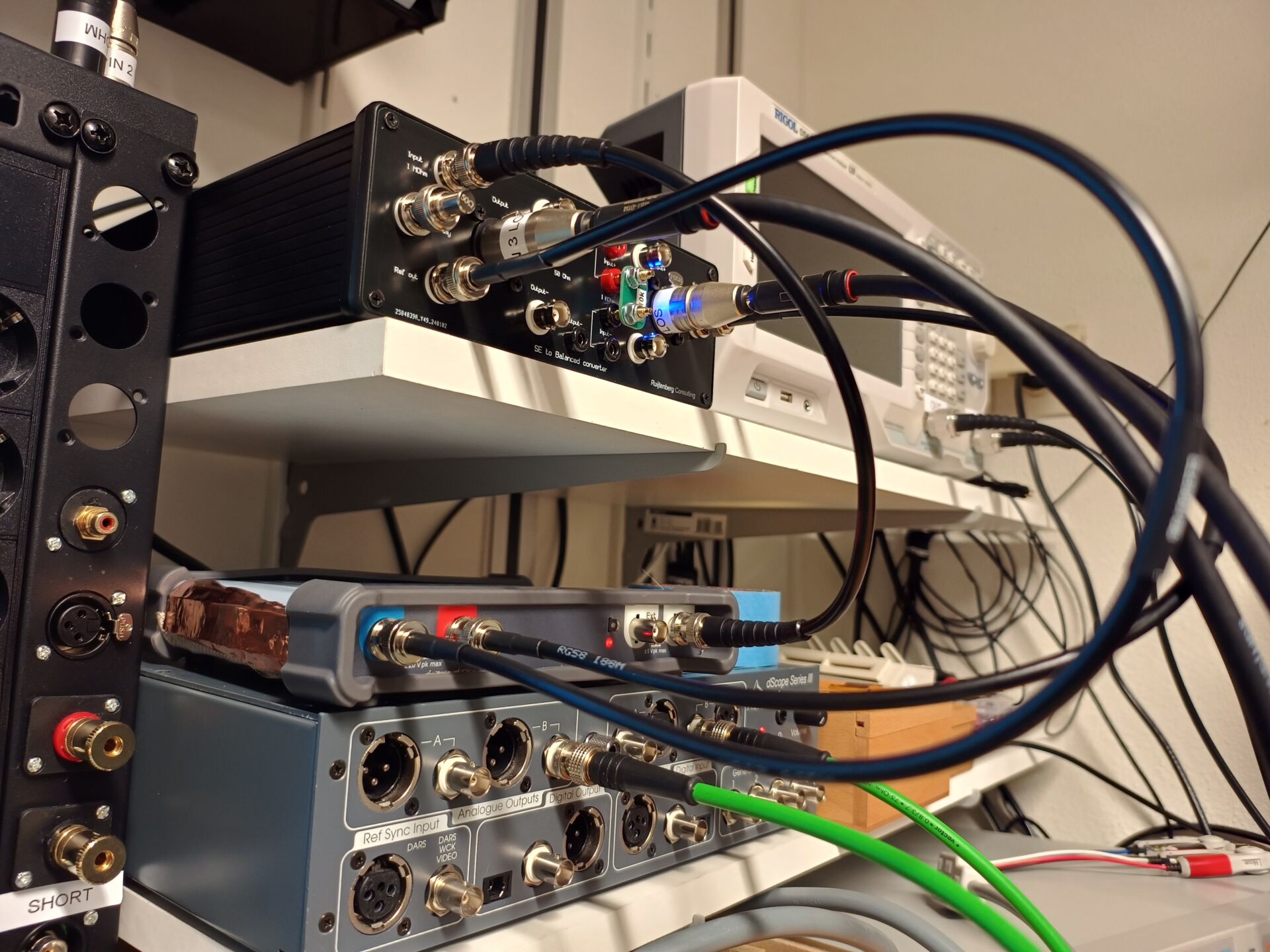
We sat down with Cees Ruijtenberg to figure out how to create a flexible and solid measurement setup. He designed a very handy little box, specifically for this test where it is possible to go from single ended inputs and outputs to balanced or banana. In other words, we can now convert from anything to anything. Extremely handy. And necessary in both this test and later the test of speaker cables.
Perhaps much more importantly: we can completely isolate the cable from the measurement setup. And that is crucial for these measurements, since otherwise we would be measuring the measuring equipment along with it. And that would extremely affect the results.
Finally, this box allows us to vary impedances on both input and output. We can do that with very handy dummies that we can simply connect to the input or output. In short: an indispensable tool in this test.


With this box, we mainly measured response and phase via the Rigol spectrum analyzer and the Picoscope 5000. In these measurements, we set the output impedance to 50 Ohms and the input impedance to 10 KOhm.
You can see above the so-called bodeplot where the blue line is the frequency response (you can see the dB on the left) and the red line is the phase (degrees on the right). The horizontal scale is frequency (logarithmic at the bodeplot). We also measured the response with our Rigol spectrum analyzer. That one allows you to superimpose measurements from three cables, which can be useful if you want to compare results. Note that this scale is linear, so it looks different from the bodeplot which shows a logarithmic scale.
Time behavior

To measure time behavior, we bought a ‘new’ used Tektronix TDS7104 scope and an HP 8131A pulse generator via Ebay. These ‘new’ devices were necessary because we simply need extremely fast equipment to map time behavior. We are (with two-meter-long cables) in the nano- and picosecond range, after all. That sounds like an idiotic thing to do, but know that human hearing is extremely sensitive to temporal behavior AND if a cable does not respond uniformly to amplitude or frequency, then it causes unrest.
Also, we just have to “magnify” things to make it visible at all. Within the audio spectrum we are not going to see time differences on a scope. However, they are there. By forcing things a bit with extremely short pulses (2ns in these tests) we can make things visible.


Above you can see a timing measurement on the Tektronix. In this case we are measuring with a 2ns pulse that we send through the cable with three voltages: 0.3V, 0.5V and 1.5V. We made the graph a little more tight by averaging.
What we are curious about is a difference in the time it takes for the pulse to pass through the cable. To do that, we plot the reference pulse (yellow) against the pulse going through the test cable (green). You can see that in the chart at the top right.
Ideally, there is no difference. In fact, if there is a difference, it would mean that the propagation time depends on the amplitude.


These two measurements show time taken by the pulse to pass through the cable. Again, we plot the reference (yellow) against the cable to be measured (green). However, we also measure the time to reflection (yellow bump after the green one) and the voltage differences between the reflections (attenuation) and the reference and the pulse through the cable.
Noise
With the Tektronix we did not only look at pulses, but we also looked at the spectrum of the cables – picture on the right – and we also looked at what the cable picks up in terms of noise. The spectrum shows how the energy dissipates after the pulse.


We made the noise pattern visible with a so-called persistence measurement. You are shown the signal in a color scale, so the scope shows how much or how strong the signal is. Ideal for making noise pickup visible.
Capacitance, inductance and impedance


Of course, we also measured all the cables with the Sourcetronic 2829A LCR meter. This sweeps from 20 Hz – 300 KHz. We set the voltage to 1 volt for this test. To get an idea of the overall characteristics, we measured capacitance, inductance, impedance (and phase) and also common resistance.


Above are three measurements of the LCR. In the impedance measurement, we add the phase.
Thank you very much for this fantastic test. Do you think the results can be applied to XLR cables?
Yes
Good morning,
This was a fascinating read and most of it was understandable.
This inspired me to make up an interconnect cable using Sommer Tricone. Switching between this and a QED QNECT2 was night and day, my ears like the difference and this has told me that swapping interconnects is worth considering.
I am jumping onto your speaker cable test next.
Thanks!
I have a question. I think it’s a language thing.
In your measurement of “impedance”, is that actually the resistance value or equivalent of the looped conductors or is it the characteristic impedance of the cable? It doesn’t seem like the latter at all, which might be very interesting to understand.
Keep up the great work!
Impedance is complex resistance.
https://en.m.wikipedia.org/wiki/Impedance
That’s actually not my question.
There’s the loop resistance/impedance of the conductors and there’s also the characteristic impedance of the transmission line.
For example, there’s 50 Ohm coaxial cable. That’s the characteristic impedance. Zip cord has a characteristic impedance of around 90 Ohms. That’s all a combination of the inductance, capacitance, resistance of the wire, and so on.
https://en.wikipedia.org/wiki/Characteristic_impedance
This value rises considerably as you go below 100 KHz.
http://k9yc.com/TransLines-LowFreq.pdf
It is just the resistance. Not the characteristic impedance.
Great! Thanks!
I’m looking forward to your speaker cable tests.
Hopefully we will have it live at the end of april.
I did wonder. In a youtube video you talk about the HP pulse generator being 500MHz generating a 2ns pulse. At 500Mhz the wavelength is about 60cm, which is shorter than te length of the cable. So you enter transmission line theory territory, and the characteristic impedance comes into play.
In the video you state that channel 1 is terminated at 50 Ohm and channel 2 at 1 Mohm (which could be considered open ended).
And in between channel 1 and 2 is the cable., with its characteristic impedance for transmission line situations, which 500MHz is I think. So every cable that does not have a characteristic impedance of 50 Ohms will cause reflections. It does not matter if the cable is good or not, it is just caused by the transmission line impedance mismatch.
The characteristic impedance of the TPR is given as 110 Ohms, which causes the reflections. I cannot find this value for the SQM, but if that would be 50 Ohm, this would explain its non-reflection-behaviour in the test.
But in audio frequency territory, this characteristic impedance is of no importance and it does not say anything about the quality of the cable.
Just a few thoughts that kept me busy 🙂 Love to hear your view on this.
Hi F.Vcp.
You are right. That’s why we didn’t do all tests on those frequencies, but did a series of tests to see what is important and what isn’t important. The ‘reflection-test’ was purely for propagation speed and -variance. Not to analyze impulse behaviour or anything. For obvious reasons, we needed a frequency that gave a shorter wavelength, for we needed to isolate the puse.
Jaap, first very well done. Probably the only way to do this better would have been if you had a reel of the cable 1000M long to determine better what the cable attributes are at 1M.
But I was talking to a good friend physics about this. Just like component differences, I think the sonic difference has to do with the designers. I always say this at a show, throw 10 designers in a room with the same parts and you get 10 different products.
In the cable realm you have metal, dielectric, insulation, wind, layout, shielding and directionality…. all these designers have their own take on what is important and that is why cables sound different.
Plus look at the variables you have on either end!
Thanks again, really great stuff!
Gordon
Hey Gordon,
I think you are right. And very nice analogy!
Hey all, there was/is an interesting exchange on this test and its results over on the Dutch side. Jaap has given me permission to use the translation I produced (Apple Translate) and repost it here for all to see. What I love about it is that this is exactly the kind of helpful result a researcher wants to see. Good research typically should generate more questions than answers, especially in its early stages. That’s normal and how the process and what it examines becomes more refined.
============================
April 6 2024 — Posted by Ad Braam (translation from Dutch) with Jaap’s responses following each question.
Jaap, upon further study I still have a number of questions (sometimes for confirmation) to be able to understand the research well. First of all, it is clear to me that the intention is to investigate whether a relationship can be found between the measurements and the listening tests and not so much to determine what is a good interlink (in my opinion very dependent on the rest of the audio system).
1. The ‘explanation of measurements’ says ‘Ideal there is no difference’. Is it meant: Ideal is there no difference when the voltage is increased from 0.3 to 1.5 volts?
A: There is ideally no difference in propagation when the voltage changes.
2. Does the voltage in an analog interlink vary between 0.3 and 1.5 volts?
A: A line output works at 2 volts at RCA. But of course the tensions vary with the music. I chose these 3 voltages to gain insight into small and large differences in amplitude.
3. Is the propagation time the difference in time it takes the pulse to go through the cable?
A: No. The propagation time is the time it takes pulse to go through the cable. So sometimes there is a difference in that when the amplitude changes.
4. How is it that the pulse that goes through the cable (green) is higher than the reference pulse (yellow)?
A: This has to do with the closure impedance, among other things. On the yellow that is 50 Ohm. On the green that’s 1 MOhm. That to imitate an exit / entrance.
5. As for noise measurements. Is it possible to explain the ‘spectral view’ in more detail. What do the green and brown lines mean? Because of this I don’t understand the statements between vd Hul and Grimm.
A: Spectral view is not noise measurement. This one displays decay. Often: extinction after a signal. Explaining this goes too far for a comment section.
6. What is the explanation that at lower frequencies the induction and capacity swings like this?
A: I don’t know exactly either. It has to do with wavelengths, among other things, but I also have to dive into this.
7. It is confusing that the vertical scale in the messenger plot is not the same when comparing Ricable and Mogami. I didn’t understand the conclusion at first.
A: You can’t do anything about that. The software scales itself and that is also necessary to keep it readable.
8. Propagation variance table very interesting. Do I understand correctly that ‘gets faster’ means that with increasing tension the propagation time becomes smaller?
A: Yes
9. Apart from the conclusions listed under the table, can you also conclude that a ‘good’ cable should have a low variance?
A: Yes. Less variation is better. Ideally it is 0.
There are a lot of questions, but hopefully I’m not the only one who has these kinds of questions.
END OF REPOST
it’s pure nonsense, what about the cheap connectors and simple wires inside a unit and i’d like to see these kind of things done by a university, not by a annoying guy which is close to the source……and all those terms:the highs are too promonent,but vague……for example, how do you know it’s not by bad wiring instead of the interlink. As an engineer micro-electronics i can say that you’re an indiot if you buy overexpensive interlinks, you’d better buy a more expensive amp
Thank you for the feedback.
Dear Richard. How do you explain the difference that is evident from the measurements of the cables?
Well, I’m a retired university researcher of 30+ years and I don’t have a problem with what these guys are doing. Is it the rigorous and pure scientific method backed up by statistical analysis? No. But I can tell you that this kind of casual but thoughtful and carefully-managed research, performed within their admitted and openly public constraints, has led to more complex and sophisticated follow-up by others quite often. After all, it is the repeated casual observations (yes, including the subjective) of others with sincere and deep interest in a subject that stimulate the start of funded research in a wide variety of fields. I would suggest to others who have the background to be helpful with ideas, money, and/or time instead of throwing bricks. We’re adults, not children. Carry on gentlemen, you’re doing fine.
Thanks Alan!
👍 I couldn’t think of a better response
I wonder if it would be possible to feed all of this tabular measurements, graphs, and subjective observations into an AI model and ask what characteristics are most correlated since it is so complex. Awesome effort guys. I can’t think of anyone else having attempted this publically. Mahalo!
Thank you! Maybe… Hmmm… Interesting thought.
Agreed
Is it fair to consider that the composite values shown in the All Data table, when coupled with the subjective observations, could hint at a kind of value proposition when MSRP is taken into account? You know…..loosely. Have to factor in the rationality of those doing the listening of course. 😉
I have looked at that as well, but haven’t found a logical link…
Regarding the rationality of the listeners or that the lowest composite value+observations:cost? Both equally…challenging I suspect. But I think there is some guidance that could be drawn or inferred from the latter.
I really tried to find a link between what we hear and what the data in ‘All Data’ says. What I did notice is that too high a capacitance or inductance is definately not good. Cables that show a decent distribution between the two mostly show a good sound balance.
The thing is: the data in that table doesn’t show the frequency response, nor the spectrum behaviour. And those two really gave insight in the performance of the cable. Along with the temporal behaviour (propagation variance).
There are other variables affecting quality. So its only part of the picture then. Not enough to guide a purchase decision. And, in the end, that’s also going to come down to buyer motivations, which is another can of worms. So I see what you’re saying. Still, this data provides a place from which you or others can build in the measurable areas. Valuable nonetheless. Well done.
Thank you. But the freq response and spectrum measurements are in this article. The thing is: they are not a simple value I can put in a table.
Good work 😉
I wish you would have done the tower and evergreen rca from Audioquest 😉
Hence my question : if someone is on a budget and need a coaxial cable , I usually advice an Audioquest forest as they are great for the money.
Is there an rca cable that you recommand also around 50€ ? Audioquest tower and evergreen would be the equivalent of the forest coaxial but they’re completely different type of cable 😉
Thanks !
(The rca are for a cd player and a rega io )
Ready the article. There are cables around €50 and less in there.
First, BIG shoutout to you guys for having the cojones to take this on. Just one look at the data sheet….HUGE undertaking. I have to think that this is a significant contribution to audiophiles everywhere who have been wondering. Perhaps it will stimulate follow-up on the part of others even. That’s what research is all about. Secondly, am I missing something? The data summary doesn’t show any values, Impedance-Inductance-Capacitance, for the Transparent Plus, yet it seems to show in its individual graphs. I’m sure you didn’t miss something so obvious, so can you explain to me? Thanks.
Hey Alan!
Thanks! I also hope that others will pick this up and make some progress. It’s needed :-).
The Transparent is sort of a weird cable. The values of impedance, capacitance and inductance are way higher due to the filter-network. If I would put them in the graphs, the scale would be messed up. That’s why I left it out.
Ah. Got it. Makes sense. Thx.